Background
This project focuses on the Exploratory Data Analysis, including data exploration, data preparation, and data cleaning. The dataset of interest here is the training dataset of Loan Prediction Problem Dataset. The original problem is to predict customers' loan eligiblity based on their application details. This project does not cover the Loan Prediction steps nor the Machine Learning algorithms.
Data Dictionary:
- Loan_ID: Unique Loan ID
- Gender: Male/Female
- Married: Applicant married Y/N
- Dependents: Number of dependents
- Education: Graduate/Undergrad
- Self_Employed: Y/N
- ApplicantIncome: Applicant Income
- CoapplicantIncome: Coapplicant Income
- LoanAmount: Loan amount in thousands
- Loan_Amount_Term: Term of loan in months
- Credit_History: 1 for meeting the guidelines, 0 for not meeting the guidelines
- Property_Area: Urban/Semi Urban/Rural
- Loan_Status: Loan approved Y/N
Loading Dataset
import pandas as pd
import seaborn as sns
from scipy.stats import chi2_contingency
from statsmodels.stats import weightstats as stests
import matplotlib.pyplot as plt
df = pd.read_csv("C:/Users/Elle/Desktop/jupyter_folder/datasets/loan_train.csv")
df.head()
Although we are not going to solve the original Loan Prediction problem here, it is generally helpful to keep the orginal problem in mind while performing the data exploration analysis. Thus the types of variables can be defined as following:
(Possible) Predictor Variable:
- Gender
- Married
- Dependents
- Education
- Self_Employed
- ApplicantIncome
- CoapplicationIncome
- LoanAmount
- Loan_Amount_Term
- Credit_History
- Property_Area
Target Variable:
- Loan_Status
# dataset comprises of 614 observations and 13 charateristics
df.shape
df.info()
Section Summary
The dataset can be separated into the following two variable categories:
Categorical:
- Gender
- Married
- Education
- Self_Employed
- Loan_Amount_Term
- Credit_History
- Property_Area
- Loan_Status
Continuous:
- ApplicantIncome
- CoapplicantIncome
- LoanAmount
Univariate Analysis
Categorical Variables
freq_tbl1 = df.groupby(['Gender','Married','Education','Self_Employed'])
freq_tbl1.size()
freq_tbl2 = df.groupby(['Credit_History','Property_Area','Loan_Amount_Term'])
freq_tbl2.size()
df.Loan_Status.value_counts()
There are more loans approved than rejected.
Continuous Variables
df[['ApplicantIncome','CoapplicantIncome','LoanAmount']].describe()
Observations:
- there are missing values on the latter characteristic
- there is notably a large difference between the 75th percentile and max values of all three variables
Thus two observations suggest that there are missing values and outliers in our data set, treatments should be applied in order to avoid building a biased predictive model.
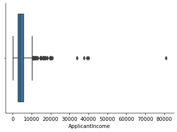
# indeed we found there are quite a few outliers
sns.boxplot(df['ApplicantIncome'])
sns.despine()
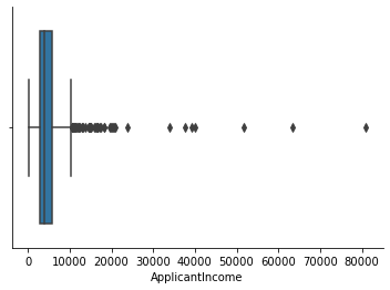
IQR_app = df.ApplicantIncome.quantile(0.75) - df.ApplicantIncome.quantile(0.25)
upper_limit_app = df.ApplicantIncome.quantile(0.75) + (IQR_app*1.5)
upper_limit_extreme_app = df.ApplicantIncome.quantile(0.75) + (IQR_app*2)
upper_limit_app, upper_limit_extreme_app
outlier_count_app = len(df[(df['ApplicantIncome'] > upper_limit_app)])
outlier_count_app
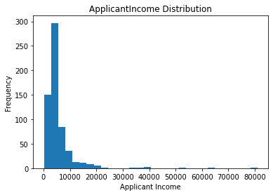
# the ApplicantIncome distribution is right skewed
fig=plt.figure()
ax=fig.add_subplot(1,1,1)
ax.hist(df['ApplicantIncome'], bins=30)
plt.title('ApplicantIncome Distribution')
plt.xlabel('Applicant Income')
plt.ylabel('Frequency')
plt.show()
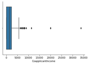
sns.boxplot(df['CoapplicantIncome'])
sns.despine()
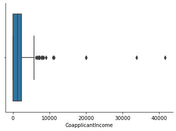
IQR_coapp = df.CoapplicantIncome.quantile(0.75) - df.CoapplicantIncome.quantile(0.25)
upper_limit_coapp = df.CoapplicantIncome.quantile(0.75) + (IQR_coapp*1.5)
upper_limit_extreme_coapp = df.CoapplicantIncome.quantile(0.75) + (IQR_coapp*2)
upper_limit_coapp, upper_limit_extreme_coapp
outlier_count_coapp = len(df[(df['CoapplicantIncome'] > upper_limit_coapp)])
outlier_count_coapp
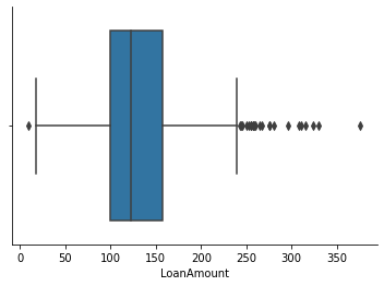
sns.boxplot(df['LoanAmount'])
sns.despine()
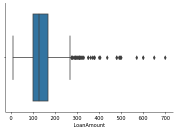
IQR_loanAmt = df.LoanAmount.quantile(0.75) - df.LoanAmount.quantile(0.25)
upper_limit_loanAmt = df.LoanAmount.quantile(0.75) + (IQR_loanAmt*1.5)
upper_limit_extreme_loanAmt = df.LoanAmount.quantile(0.75) + (IQR_loanAmt*2)
upper_limit_loanAmt, upper_limit_extreme_loanAmt
outlier_count_loanAmt = len(df[(df['LoanAmount'] > upper_limit_loanAmt)])
outlier_count_loanAmt
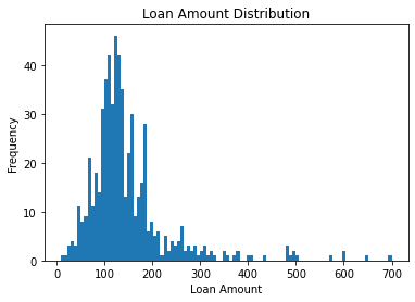
# the LoanAmount distribution is right skewed
fig=plt.figure()
ax=fig.add_subplot(1,1,1)
ax.hist(df['LoanAmount'], bins=100)
plt.title('Loan Amount Distribution')
plt.xlabel('Loan Amount')
plt.ylabel('Frequency')
plt.show()
Section Summary
Variables with missing values:
- Gender (13 or 2.1%)
- Married (3 or 0.5%)
- Dependents (15 or 2.4%)
- Self_Employed (32 or 5.2%)
- LoanAmount (22 or 3.6%)
- Loan_Amount_Term (14 or 2.3%)
- Credit_History (50 or 8.1%)
Variables with outliers:
- ApplicantIncome (43 outliers exceeding its maximum value)
- CoapplicantIncome ( 17 outliers exceeding its maximum value)
- LoanAmount (30 outliers exceeding its maximum value)
where "Maximum" refers to 75th Percentile + 1.5$$(Interqartile Range)*
Bivariate Analysis
Categorical and Categorical
Loan_Status and Gender
tbl = pd.crosstab(index = df['Loan_Status'], columns = df['Gender'])
tbl.index = ['Not Approved','Approved']
tbl
Pearson's Chi-square Test
The chi-square test statistic for a test of independence of two categorical variables is as follows: $$ \begin{aligned} \chi^2 = \sum{(O - E)^2 / E} \;, \;Where\:O \:is \:the \:observed \:frequency \:and \\\:E \:is \:the \:expected \:frequency \end{aligned} $$
$ \\ H_0: \:There \:is \:no \:relationship \:between \:Loan\:Status \:and \:Gender \\H_1: \:There \:is \:a \:significant \:relation \:between \:the \:two $
Calculated chi-square value (orginal frequency table excluding missing values)
The calculated $\chi^2$ value is 0.2369751, where the degree of freedom is 1. The critical value of the $\chi^2$ distribution with df of 1 is 3.841.
Hence:
$$ \begin{aligned} critical\:value\:of\:\chi^2\: >=\:calculated\:value\:of\:\chi^2 \end{aligned} $$Therefore $H_0$ is Accepted
# performing the test using Python
# frequency table without missing values
stat, p, dof, expected = chi2_contingency(tbl)
alpha = 0.05
print("p value is " + str(p))
if p <= alpha:
    print('Dependent (reject H_0)')
else:
    print('Independent (H_0 holds true)')
# How would the table look like if we include counts of missing-value obersvations?
tbl2 = tbl
df_new = df[df['Gender'].isnull()]
tbl_tp = df_new.groupby('Loan_Status')
tbl_tp.size()
tbl2['NaN_val'] = [5,8]
tbl2
tbl2.plot.bar(xlabel = 'Loan Status', rot = 0)
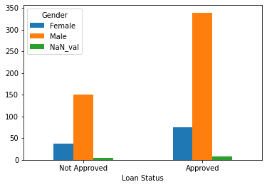
The above bar plot does not provide much evidence to show that there is a significant relationship between Loan_Status and Gender.
Calculated chi-square value (modified frequency table including counts of missing values)
The calculated $\chi^2$ value is 5.66887, where the degree of freedom is 2. The critical value of the $\chi^2$ distribution with df of 2 is 5.991.
Hence:
$$ \begin{aligned} critical\:value\:of\:\chi^2\: >=\:calculated\:value\:of\:\chi^2 \end{aligned} $$Therefore $H_0$ is Accepted
# performing the test using Python
# frequency table with missing values
stat, p, dof, expected = chi2_contingency(tbl2)
alpha = 0.05
print("p value is " + str(p))
if p <= alpha:
    print('Dependent (reject H_0)')
else:
    print('Independent (H_0 holds true)')
Both $\chi^2$ tests reject the $H_0$, sugguesting that there is no significant relationship between Loan_Status and Gender.
Loan_Status and Married
tbl_marrd = pd.crosstab(index = df['Loan_Status'], columns = df['Married'])
tbl_marrd.index = ['Not Approved','Approved']
tbl_marrd.columns = ['Not Married','Married']
tbl_marrd
Chi-square Test
$ H_0: \:There \:is \:no \:relationship \:between \:variables\:Loan\:Status\:and\:Married \\H_1:\: Negation\:of\:H_0 $
stat, p, dof, exptected = chi2_contingency(tbl_marrd)
alpha = 0.05
print("p value is " + str(p))
if p <= alpha:
    print('Dependent (reject H_0)')
else:
    print('Independent (H_0 holds true)')
Loan_Status and Education
tbl_ed = pd.crosstab(df['Loan_Status'],df['Education'])
tbl_ed.index = ['Not Approved','Approved']
tbl_ed
tbl_ed.plot.bar(xlabel = 'Loan Status', rot = 0)
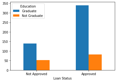
Chi-square Test
$ H_0: \:There \:is \:no \:relationship \:between \:Loan\:Status\:and\:Education \\H_1:\: Negation\:of\:H_0 $
stat, p, dof, exptected = chi2_contingency(tbl_ed)
alpha = 0.05
print("p value is " + str(p))
if p <= alpha:
    print('Dependent (reject H_0)')
else:
    print('Independent (H_0 holds true)')
The above probability indicates that the relationship between Loan_Status and Education is significant at 95% confidence.
Loan_Status and Self_Employed
tbl_emp = pd.crosstab(index = df['Loan_Status'], columns = df['Self_Employed'])
tbl_emp.index = ['Not Approved','Approved']
tbl_emp
Self_Employed has 32 missing values.
tbl_emp.plot.bar(xlabel = 'Loan Status',rot = 0)
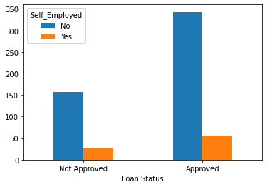
Chi-square Test
$ H_0: \:There \:is \:no \:relationship \:between \:Loan\:Status\:and\:Self\_Employed \\H_1:\: Negation\:of\:H_0 $
stat, p, dof, expected = chi2_contingency(tbl_emp)
alpha = 0.05
print("p value is " + str(p))
if p <= alpha:
    print('Dependent (reject H_0)')
else:
    print('Independent (H_0 holds true)')
Chi-square test sugguests that there is no significant relationship between Loan_Status and Self_Employed.
Loan_Status and Loan_Amount_Term
tbl_term = pd.crosstab(index = df['Loan_Status'], columns = df['Loan_Amount_Term'])
tbl_term.index = ['Not Approved','Approved']
tbl_term
stat, p, dof, exptected = chi2_contingency(tbl_term)
alpha = 0.05
print("p value is " + str(p))
if p <= alpha:
    print('Dependent (reject H_0)')
else:
    print('Independent (H_0 holds true)')
Loan_Status and Credit_History
tbl_crt = pd.crosstab(index = df['Loan_Status'], columns = df['Credit_History'])
tbl_crt.index = ['Not Approved','Approved']
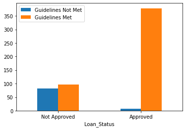
tbl_crt.columns = ['Guidelines Not Met', 'Guidelines Met']
tbl_crt
- Credit_History has 50 missing values
- It seems to suggest that there are relatively more loans approved when the applicants' credit meets the guidelines
tbl_crt.plot.bar(xlabel = 'Loan_Status', rot = 0)
Chi-square Test
$ H_0: \:There \:is \:no \:relationship \:between \:Loan\:Status\:and\:Credit\_History \\H_1:\: Negation\:of\:H_0 $
stat, p, dof, expected = chi2_contingency(tbl_crt)
alpha = 0.05
print("p value is " + str(p))
if p <= alpha:
    print('Dependent (reject H_0)')
else:
    print('Independent (H_0 holds true)')
Loan_Status and Property_Area
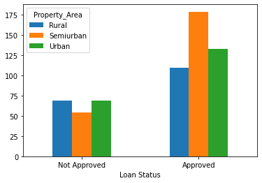
tbl_area = pd.crosstab(index = df['Loan_Status'], columns = df['Property_Area'])
tbl_area.index = ['Not Approved','Approved']
tbl_area
tbl_area.plot.bar(xlabel = 'Loan Status', rot = 0)
Chi-square Test
$ H_0: \:There \:is \:no \:relationship \:between \:Loan\:Status\:and\:Property\_Area \\H_1:\: Negation\:of\:H_0 $
stat, p, dof, exptected = chi2_contingency(tbl_area)
alpha = 0.05
print("p value is " + str(p))
if p <= alpha:
    print('Dependent (reject H_0)')
else:
    print('Independent (H_0 holds true)')
Categorical and Continuous
Loan_Status and ApplicantIncome
df['ApplicantIncome'].groupby(df['Loan_Status']).describe()
# data set of Loan_Status Not Approved
tbl_appN = df[(df['Loan_Status'] == 'N')]
tbl_appN = tbl_appN['ApplicantIncome']
tbl_appN
# data set of Loan_Status Approved
tbl_appY = df[(df['Loan_Status'] == 'Y')]
tbl_appY = tbl_appY['ApplicantIncome']
tbl_appY
Two sample Z-Test (ApplicantIncome splitted by Loan_Status)
$$ H_0: \:\mu_{N_{income}} =\:\mu_{Y_{income}} \\H_1:\: Negation\:of\:H_0 $$Assuming two levels of samples are independent.
ztest, pval = stests.ztest(tbl_appN,tbl_appY,value = 0, alternative = 'two-sided')
alpha = 0.05
print("p value is " + str(pval))
if pval <= alpha:
    print('Two population means are not equal (reject H_0)')
else:
    print('Two population means are equal (H_0 holds true)')
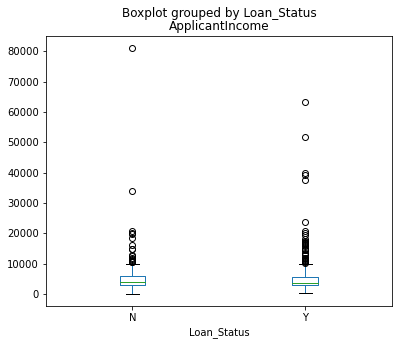
Conclusion
There is no evidence that the difference in Applicant income will have an impact on loan eligibility.
fig, ax = plt.subplots(figsize = (6,5))
df.boxplot(column = 'ApplicantIncome', by = 'Loan_Status', ax = ax, grid = False)
plt.show()
Loan_Status and LoanAmount
df['LoanAmount'].groupby(df['Loan_Status']).describe()
tbl_amtN = df[(df['Loan_Status'] == 'N')]
tbl_amtN = tbl_amtN['LoanAmount'].dropna() # we know there are missing values
tbl_amtN
tbl_amtY = df[(df['Loan_Status'] == 'Y')]
tbl_amtY = tbl_amtY['LoanAmount'].dropna() # missing values dropped
tbl_amtY
Two sample Z-Test (LoanAmount splitted by Loan_Status)
$$ H_0: \:\mu_{N_{LoanAmt}} =\:\mu_{Y_{LoanAmt}} \\H_1:\: Negation\:of\:H_0 $$Assuming two levels of samples are independent.
ztest, pval = stests.ztest(tbl_amtN,tbl_amtY,value = 0, alternative = 'two-sided')
alpha = 0.05
print("p value is " + str(pval))
if pval <= alpha:
    print('Two population means are not equal (reject H_0)')
else:
    print('Two population means are equal (H_0 holds true)')
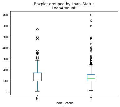
Conclusion
There is no evidence that the difference in Loan Amount will result in lower/higher loan acceptance rate.
fig, ax = plt.subplots(figsize = (6,5))
df.boxplot(column = 'LoanAmount', by = 'Loan_Status', ax = ax, grid = False)
plt.show()
Continuous and Contintuous
ApplicantIncome vs. LoanAmount
fig = plt.figure()
ax = fig.add_subplot(1,1,1)
ax.scatter(df['ApplicantIncome'],df['LoanAmount'])
plt.title('ApplicantIncome and LoanAmount Distribution')
plt.xlabel('Applicant Income')
plt.ylabel('Loan Amount')
plt.show()
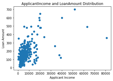
From the above scatter plot, it looks like there is a positive correlation between 'LoanAmount' and 'ApplicantIncome'. Yet here we have not performed any missing data nor outlier treatment, thus it is too early to make a conclusion.
CoapplicantIncome vs. LoanAmount
fig = plt.figure()
ax = fig.add_subplot(1,1,1)
ax.scatter(df['CoapplicantIncome'],df['LoanAmount'])
plt.title('CoapplicantIncome and LoanAmount Distribution')
plt.xlabel('Coapplicant Income')
plt.ylabel('Loan Amount')
plt.show()
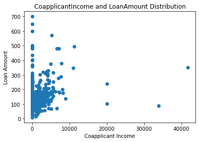
It is hard to make any conclusion from the above scatter plot, but it looks like a portion of the points sugguests the positive correlation. Ideally to double check, we would calculate the correlation coefficient, but due to difference in two variables' shapes, we have to perform missing values treatment in order to proceed with correlation calculation.
Section Summary (where the missing values are simply ignored)
Predictor variables that are observed to have a statistacally significant association with the Target varialbe are as follows:
- Married
- Education
- Credit_History
- Property_Area
Missing value Treatment
From previous analysis, we know most of the variables have at least one missing value, below will examine the possible cause of the occurence of the missing values, in my opinion, for each variable.
- Gender: Most likely be missing completely at random(MCAR)
- Married: MCAR
- Dependents: MCAR
- Self_Employed: MCAR
- LoanAmount: MCAR
- Loan_Amount_Term: MCAR
- Credit_History: Missing at random. Applicants who do not meeting credit guidelines tend to have higher missing value compare to those whose credit met the guidelines.
Statistically speaking, if the number of missing observations is less than 5% of the sample, we can drop them. In addition, if the missing value is determined to be MCAR, we can safely perform deletion of missing value cases. With that said, missing observations of Gender, Married, Dependents, Self_Employed, LoanAmount and Loan_Amount_Term can be dropped.
As for Credit_History, imputation will be conducted to replace the missing ones.
Credit_History Imputation
Before the actual imputation, we should examine if there's any correlation between Credit_History and other variables.
Credit_history vs Gender
Chi-square Test
$ H_0: \:There \:is \:no \:relationship \:between \:variables\:Credit\_History\:and\:Gender \\H_1:\: Negation\:of\:H_0 $
tbl_cGender = pd.crosstab(df['Credit_History'],df['Gender'])
stat, p, dof, exptected = chi2_contingency(tbl_cGender)
alpha = 0.05
print("p value is " + str(p))
if p <= alpha:
    print('Dependent (reject H_0)')
else:
    print('Independent (H_0 holds true)')
Credit_History vs Married
Chi-square Test
$ H_0: \:There \:is \:no \:relationship \:between \:variables\:Credit\_History\:and\:Married \\H_1:\: Negation\:of\:H_0 $
tbl_cMarried = pd.crosstab(df['Credit_History'],df['Married'])
stat, p, dof, exptected = chi2_contingency(tbl_cMarried)
alpha = 0.05
print("p value is " + str(p))
if p <= alpha:
    print('Dependent (reject H_0)')
else:
    print('Independent (H_0 holds true)')
Credit_History vs Education
Chi-square Test
$ H_0: \:There \:is \:no \:relationship \:between \:variables\:Credit\_History\:and\:Education \\H_1:\: Negation\:of\:H_0 $
tbl_cEd = pd.crosstab(df['Credit_History'],df['Education'])
stat, p, dof, exptected = chi2_contingency(tbl_cEd)
alpha = 0.05
print("p value is " + str(p))
if p <= alpha:
    print('Dependent (reject H_0)')
else:
    print('Independent (H_0 holds true)')
Credit_History vs Self_Employed
Chi-square Test
$ H_0: \:There \:is \:no \:relationship \:between \:variables\:Credit\_History\:and\:Self\_Employed \\H_1:\: Negation\:of\:H_0 $
tbl_cEmp = pd.crosstab(df['Credit_History'],df['Self_Employed'])
stat, p, dof, exptected = chi2_contingency(tbl_cEmp)
alpha = 0.05
print("p value is " + str(p))
if p <= alpha:
    print('Dependent (reject H_0)')
else:
    print('Independent (H_0 holds true)')
Credit_History vs Property_Area
Chi-square Test
$ H_0: \:There \:is \:no \:relationship \:between \:variables\:Credit\_History\:and\:Property\_Area \\H_1:\: Negation\:of\:H_0 $
tbl_cArea = pd.crosstab(df['Credit_History'],df['Property_Area'])
stat, p, dof, exptected = chi2_contingency(tbl_cArea)
alpha = 0.05
print("p value is " + str(p))
if p <= alpha:
    print('Dependent (reject H_0)')
else:
    print('Independent (H_0 holds true)')
Credit_History vs ApplicantIncome
Two sample Z-Test (ApplicantIncome splitted by Loan_Status)
$$ H_0: \:\mu_{N_{applicantIncome}} =\:\mu_{Y_{applicantIncome}} \\H_1:\: Negation\:of\:H_0 $$df['ApplicantIncome'].groupby(df['Credit_History']).describe()
tbl_incomeN = df[(df['Credit_History'] == 0.0)]
tbl_incomeN = tbl_incomeN['ApplicantIncome']
tbl_incomeN
tbl_incomeY = df[(df['Credit_History'] == 1.0)]
tbl_incomeY = tbl_incomeY['ApplicantIncome']
tbl_incomeY
ztest, pval = stests.ztest(tbl_incomeN,tbl_incomeY,value = 0, alternative = 'two-sided')
alpha = 0.05
print("p value is " + str(pval))
if pval <= alpha:
    print('Two population means are not equal (reject H_0)')
else:
    print('Two population means are equal (H_0 holds true)')
Observation: There isn't any correlation between Credit_History and other predictor variables.
Imputation using Most Frequent values
import numpy as np
from sklearn.impute import SimpleImputer
imr = SimpleImputer(missing_values = np.nan,strategy = 'most_frequent')
imr = imr.fit(df[['Credit_History']])
df['Credit_History'] = imr.transform(df[['Credit_History']]).ravel()
df.info()
Deletion
For simplicity, we will delete observations where any of the variables is missing due to MCAR.
# if proceed with dropping NaN before imputation
# the sample size will reduce down to 480
# yet if we drop observations where missing values are found after imputation
# the sample size is reduced to 523 rather
df = df.dropna()
df.info()
Outlier Treatment
From previous analysis, where we ignored the missing-value observations, variables ApplicantIncome, CoapplicantIncome, and LoanAmount are found to have univariate outliers in the upper boundaries. Now let's see if there's any changes on outliers after our missing value treatment.
df[['ApplicantIncome','CoapplicantIncome','LoanAmount']].describe()
sns.boxplot(df['ApplicantIncome'])
sns.despine()
IQR_1 = df.ApplicantIncome.quantile(0.75) - df.ApplicantIncome.quantile(0.25)
upper_limit_1 = df.ApplicantIncome.quantile(0.75) + (IQR_1*1.5)
upper_limit_extreme_1 = df.ApplicantIncome.quantile(0.75) + (IQR_1*2)
upper_limit_1, upper_limit_extreme_1
outlier_count_1 = len(df[(df['ApplicantIncome'] > upper_limit_1)])
outlier_count_1
# notice the number of the outliers did not change after missing-value treatment
Trimming
We will use Trimming here as our outlier treatment method.
pd.set_option('mode.chained_assignment', None)
index_1 = df[(df['ApplicantIncome'] >= upper_limit_1)].index
#index_1
df.drop(index_1, inplace = True)
outlier_ct_1 = len(df[(df['ApplicantIncome'] > upper_limit_1)])
outlier_ct_1
sns.boxplot(df['CoapplicantIncome'])
sns.despine()
IQR_2 = df.CoapplicantIncome.quantile(0.75) - df.CoapplicantIncome.quantile(0.25)
upper_limit_2 = df.CoapplicantIncome.quantile(0.75) + (IQR_2*1.5)
upper_limit_extreme_2 = df.CoapplicantIncome.quantile(0.75) + (IQR_2*2)
upper_limit_2, upper_limit_extreme_2
outlier_count_2 = len(df[(df['CoapplicantIncome'] > upper_limit_2)])
outlier_count_2
# number of outliers reduced from 17 to 16 after missing-value treatment
#pd.set_option('mode.chained_assignment', None)
index_2 = df[(df['CoapplicantIncome'] >= upper_limit_2)].index
#index_2
df.drop(index_2, inplace = True)
outlier_ct_2 = len(df[(df['CoapplicantIncome'] > upper_limit_2)])
outlier_ct_2
sns.boxplot(df['LoanAmount'])
sns.despine()
IQR_3 = df.LoanAmount.quantile(0.75) - df.LoanAmount.quantile(0.25)
upper_limit_3 = df.LoanAmount.quantile(0.75) + (IQR_3*1.5)
upper_limit_extreme_3 = df.LoanAmount.quantile(0.75) + (IQR_3*2)
upper_limit_3, upper_limit_extreme_3
outlier_count_3 = len(df[(df['LoanAmount'] > upper_limit_3)])
outlier_count_3
# number of outliers reduced from 30 to 23 after missing-value treatment
#pd.set_option('mode.chained_assignment', None)
index_3 = df[(df['LoanAmount'] >= upper_limit_3)].index
#index_3
df.drop(index_3, inplace = True)
outlier_ct_3 = len(df[(df['LoanAmount'] > upper_limit_3)])
outlier_ct_3
Variable Correlations After Data Cleaning
#encoding to numeric data type
code_numeric = {'Male':1, 'Female':2,
               'Yes': 1, 'No':2,
                'Graduate':1, 'Not Graduate':2,
                'Urban':1, 'Semiurban':2, 'Rural':3,
                'Y':1, 'N':0,
                '3+':3 }
df = df.applymap(lambda i: code_numeric.get(i) if i in code_numeric else i)
df['Dependents'] = pd.to_numeric(df.Dependents)
df.info()
matrix = np.triu(df.corr())
fig, ax = plt.subplots(figsize = (10,10))
sns.heatmap(df.corr(), annot = True, mask = matrix, linewidths = .5, ax = ax)
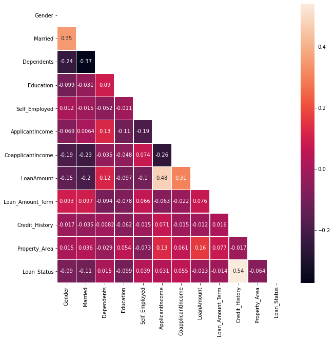
Conclusion
Depending on different methods of missing-value and/or outlier treatments, the level of data loss might have impact on prediction models which are used to solve the original problem. This project is only to explore the dataset and to describe dataset characterizations through data visualization and statistical techniques. Below shows how much each variable correlates with the target variable.
m = matrix[:,11]
m = pd.DataFrame(m)
m1 = np.transpose(m)
m1.columns = (df.columns[1:])
m2 = np.transpose(m1)
new_col = ['corr_to_Loan_Status']
m2.columns =new_col
# sort predictor variables by their correlation strength to the Target variable
m2['corr_to_Loan_Status'] = m2['corr_to_Loan_Status'].abs()
m2.sort_values(by = new_col, ascending = False)