Model Evaluation on Loan Prediction Dataset

Author: Zhanglin Liu

Date: 11/07/2020

Background

The dataset of interest here is the training dataset of the Loan Prediction Problem Dataset, which can be found on Kaggle's publicly available repository. The goal of this project is to evaluate the Logistic Regression prediction model on Loan Prediction training dataset, fine-tune the model on the validation dataset, and use appropriate and accurate diagnotics for the data.

Data Dictionary:

  • Loan_ID: Unique Loan ID
  • Gender: Male/Female
  • Married: Applicant married Y/N
  • Dependents: Number of dependents
  • Education: Graduate/Undergrad
  • Self_Employed: Y/N
  • ApplicantIncome: Applicant Income
  • CoapplicantIncome: Coapplicant Income
  • LoanAmount: Loan amount in thousands
  • Loan_Amount_Term: Term of loan in months
  • Credit_History: 1 for meeting the guidelines, 0 for not meeting the guidelines
  • Property_Area: Urban/Semi Urban/Rural
  • Loan_Status: Loan approved Y/N

Loading Dataset

In [1]:
import pandas as pd
import numpy as np
from collections import Counter
from pandas import DataFrame, Series
from sklearn.linear_model import LogisticRegression
from sklearn.metrics import confusion_matrix
from sklearn.metrics import precision_score
from sklearn.metrics import recall_score
from sklearn.model_selection import GridSearchCV
from sklearn.model_selection import RepeatedStratifiedKFold
df = pd.read_csv("loan_train.csv")
df
Out[1]:
Loan_ID Gender Married Dependents Education Self_Employed ApplicantIncome CoapplicantIncome LoanAmount Loan_Amount_Term Credit_History Property_Area Loan_Status
0 LP001002 Male No 0 Graduate No 5849 0.0 NaN 360.0 1.0 Urban Y
1 LP001003 Male Yes 1 Graduate No 4583 1508.0 128.0 360.0 1.0 Rural N
2 LP001005 Male Yes 0 Graduate Yes 3000 0.0 66.0 360.0 1.0 Urban Y
3 LP001006 Male Yes 0 Not Graduate No 2583 2358.0 120.0 360.0 1.0 Urban Y
4 LP001008 Male No 0 Graduate No 6000 0.0 141.0 360.0 1.0 Urban Y
... ... ... ... ... ... ... ... ... ... ... ... ... ...
609 LP002978 Female No 0 Graduate No 2900 0.0 71.0 360.0 1.0 Rural Y
610 LP002979 Male Yes 3+ Graduate No 4106 0.0 40.0 180.0 1.0 Rural Y
611 LP002983 Male Yes 1 Graduate No 8072 240.0 253.0 360.0 1.0 Urban Y
612 LP002984 Male Yes 2 Graduate No 7583 0.0 187.0 360.0 1.0 Urban Y
613 LP002990 Female No 0 Graduate Yes 4583 0.0 133.0 360.0 0.0 Semiurban N

614 rows × 13 columns

Data Cleaning

In [2]:
df.info()
<class 'pandas.core.frame.DataFrame'>
RangeIndex: 614 entries, 0 to 613
Data columns (total 13 columns):
 #   Column             Non-Null Count  Dtype  
---  ------             --------------  -----  
 0   Loan_ID            614 non-null    object 
 1   Gender             601 non-null    object 
 2   Married            611 non-null    object 
 3   Dependents         599 non-null    object 
 4   Education          614 non-null    object 
 5   Self_Employed      582 non-null    object 
 6   ApplicantIncome    614 non-null    int64  
 7   CoapplicantIncome  614 non-null    float64
 8   LoanAmount         592 non-null    float64
 9   Loan_Amount_Term   600 non-null    float64
 10  Credit_History     564 non-null    float64
 11  Property_Area      614 non-null    object 
 12  Loan_Status        614 non-null    object 
dtypes: float64(4), int64(1), object(8)
memory usage: 62.5+ KB
In [3]:
# drop Loan_ID column
df = df.drop(['Loan_ID'], axis = 1)
In [4]:
# Identify the columns with null values
df.isnull().sum()
Out[4]:
Gender               13
Married               3
Dependents           15
Education             0
Self_Employed        32
ApplicantIncome       0
CoapplicantIncome     0
LoanAmount           22
Loan_Amount_Term     14
Credit_History       50
Property_Area         0
Loan_Status           0
dtype: int64
In [5]:
# Fill in all null values appropriately
for col in df.columns:
    df[col].fillna(df[col].mode()[0], inplace = True)
df['LoanAmount'].fillna(df['LoanAmount'].mean(), inplace = True)
df.isnull().sum()
Out[5]:
Gender               0
Married              0
Dependents           0
Education            0
Self_Employed        0
ApplicantIncome      0
CoapplicantIncome    0
LoanAmount           0
Loan_Amount_Term     0
Credit_History       0
Property_Area        0
Loan_Status          0
dtype: int64
In [6]:
# One-hot encoding
code_numeric = {'Male':1, 'Female':2,
               'Yes': 1, 'No':2,
                'Graduate':1, 'Not Graduate':2,
                'Urban':1, 'Semiurban':2, 'Rural':3,
                'Y':1, 'N':0,
                '3+':3 }
df = df.applymap(lambda i: code_numeric.get(i) if i in code_numeric else i)
df['Dependents'] = pd.to_numeric(df.Dependents)
df.info()
<class 'pandas.core.frame.DataFrame'>
RangeIndex: 614 entries, 0 to 613
Data columns (total 12 columns):
 #   Column             Non-Null Count  Dtype  
---  ------             --------------  -----  
 0   Gender             614 non-null    int64  
 1   Married            614 non-null    int64  
 2   Dependents         614 non-null    int64  
 3   Education          614 non-null    int64  
 4   Self_Employed      614 non-null    int64  
 5   ApplicantIncome    614 non-null    int64  
 6   CoapplicantIncome  614 non-null    float64
 7   LoanAmount         614 non-null    float64
 8   Loan_Amount_Term   614 non-null    float64
 9   Credit_History     614 non-null    float64
 10  Property_Area      614 non-null    int64  
 11  Loan_Status        614 non-null    int64  
dtypes: float64(4), int64(8)
memory usage: 57.7 KB
In [7]:
# shuffle the dataset as all records should be independent of each other
df.sample(frac = 1)
Out[7]:
Gender Married Dependents Education Self_Employed ApplicantIncome CoapplicantIncome LoanAmount Loan_Amount_Term Credit_History Property_Area Loan_Status
326 1 2 0 1 2 4917 0.0 130.0 360.0 0.0 3 1
180 1 1 1 1 2 6400 7250.0 180.0 360.0 0.0 1 0
56 1 1 0 1 2 2132 1591.0 96.0 360.0 1.0 2 1
472 1 1 3 1 2 4691 0.0 100.0 360.0 1.0 2 1
609 2 2 0 1 2 2900 0.0 71.0 360.0 1.0 3 1
... ... ... ... ... ... ... ... ... ... ... ... ...
194 1 2 0 1 2 4191 0.0 120.0 360.0 1.0 3 1
163 1 1 2 1 2 4167 1447.0 158.0 360.0 1.0 3 1
123 1 1 2 1 2 2957 0.0 81.0 360.0 1.0 2 1
186 1 1 1 1 1 2178 0.0 66.0 300.0 0.0 3 0
97 1 1 0 1 2 1977 997.0 50.0 360.0 1.0 2 1

614 rows × 12 columns

In [8]:
# separating features and target
y = df['Loan_Status']
X = df.drop(['Loan_Status'], axis = 1)
In [9]:
# Split the dataset at 60/20/20 ratio
N = len(X)
X_train = X[:3*N//5]
X_validation = X[3*N//5:4*N//5]
X_test = X[4*N//5:]
y_train = y[:3*N//5]
y_validation = y[3*N//5:4*N//5]
y_test = y[4*N//5:]
len(X),len(X_train), len(X_validation), len(X_test)
Out[9]:
(614, 368, 123, 123)
In [10]:
len(y),len(y_train), len(y_validation), len(y_test)
Out[10]:
(614, 368, 123, 123)

Prediction Model

In [11]:
# Logistic Regression model
model = LogisticRegression(max_iter = 4000)
model.fit(X_train, y_train)
print('Model Score with all features: \n', model.score(X_train, y_train))
Model Score with all features: 
 0.7880434782608695
In [12]:
print('Coefficient: \n', model.coef_)
print('Intercept: \n', model.intercept_)
Coefficient: 
 [[ 1.36883904e-01 -1.46079349e-01 -1.42282797e-02 -3.00144038e-01
   5.56749245e-01  1.71173087e-05  6.61155418e-05 -2.88458774e-03
  -4.64137684e-03  2.57582074e+00 -2.45759060e-01]]
Intercept: 
 [0.29113768]
In [13]:
coeff = DataFrame(X_train.columns)
coeff['Coefficient Estimates'] = Series(model.coef_.flatten())
coeff.columns = ['Features','Coefficient Estimates' ]
coeff
Out[13]:
Features Coefficient Estimates
0 Gender 0.136884
1 Married -0.146079
2 Dependents -0.014228
3 Education -0.300144
4 Self_Employed 0.556749
5 ApplicantIncome 0.000017
6 CoapplicantIncome 0.000066
7 LoanAmount -0.002885
8 Loan_Amount_Term -0.004641
9 Credit_History 2.575821
10 Property_Area -0.245759

Model Evaluation

In [14]:
# getting the probabilities of whether an event is happening or not 
# for each observations in X_train
prob = model.predict_proba(X_train)
# obtaining the probabilities of event happening for all observations
p_x_val = prob[:,1]
p_x_val
Out[14]:
array([0.79614169, 0.74223928, 0.74243871, 0.78722563, 0.78656791,
       0.68335155, 0.78925635, 0.20619012, 0.8039015 , 0.80732366,
       0.83550295, 0.82864181, 0.85038485, 0.73253232, 0.9470967 ,
       0.79126056, 0.83535585, 0.27097126, 0.65988969, 0.84535762,
       0.2157884 , 0.78674621, 0.17784428, 0.14427753, 0.78850137,
       0.63752538, 0.79472631, 0.7772402 , 0.77416177, 0.79031243,
       0.81068791, 0.80986518, 0.57943046, 0.79412731, 0.63724472,
       0.82975825, 0.27079503, 0.80050261, 0.83556915, 0.71496304,
       0.80833672, 0.82974443, 0.82909121, 0.79315913, 0.66841272,
       0.82488391, 0.84683735, 0.80825666, 0.31909978, 0.78634107,
       0.76829003, 0.76962265, 0.7770991 , 0.80510078, 0.13197652,
       0.78983856, 0.79793975, 0.74584932, 0.81877596, 0.77850383,
       0.84580621, 0.81427817, 0.17688633, 0.16957957, 0.20757354,
       0.7624746 , 0.35622383, 0.73580042, 0.88166129, 0.19860882,
       0.81993928, 0.62236777, 0.81265668, 0.16762008, 0.64044138,
       0.68775609, 0.81441161, 0.74707999, 0.26272126, 0.60692084,
       0.77645954, 0.65307232, 0.82187677, 0.7302225 , 0.9021402 ,
       0.76461651, 0.74721468, 0.80083679, 0.75937331, 0.79849063,
       0.79789517, 0.90501159, 0.79714833, 0.74676837, 0.89717853,
       0.79872144, 0.80924571, 0.81217915, 0.85618604, 0.80139677,
       0.8972277 , 0.77929908, 0.83780193, 0.8144328 , 0.803466  ,
       0.82808515, 0.79361389, 0.64476169, 0.23688683, 0.6042151 ,
       0.78702329, 0.80984664, 0.15208573, 0.67038375, 0.75188394,
       0.85816563, 0.80321542, 0.83553462, 0.73008826, 0.76428476,
       0.73439811, 0.80905741, 0.30128131, 0.78536529, 0.64792977,
       0.74052126, 0.63654638, 0.72016951, 0.35803049, 0.73338667,
       0.26209163, 0.82591311, 0.76980811, 0.88624828, 0.75990989,
       0.77036141, 0.77486206, 0.76916078, 0.16049843, 0.67451337,
       0.71603203, 0.77144651, 0.77824795, 0.79206953, 0.90232105,
       0.84469785, 0.87162849, 0.8549839 , 0.70807198, 0.78350266,
       0.15552725, 0.63640223, 0.74296586, 0.65643112, 0.82051694,
       0.21074651, 0.70886667, 0.79642223, 0.72301026, 0.77267579,
       0.73625345, 0.7496962 , 0.21536621, 0.72025366, 0.92643341,
       0.73316207, 0.76046004, 0.76004842, 0.12857703, 0.73890172,
       0.69780699, 0.7020528 , 0.82951574, 0.8082829 , 0.62805222,
       0.75362545, 0.747475  , 0.15496901, 0.77277603, 0.12100937,
       0.31736156, 0.78433968, 0.90135007, 0.78981904, 0.80156466,
       0.83060822, 0.14698177, 0.78207234, 0.64181939, 0.84758191,
       0.68176155, 0.7493145 , 0.74951989, 0.77019882, 0.69898167,
       0.77353202, 0.7247245 , 0.78380486, 0.82696711, 0.73115761,
       0.75850714, 0.16297924, 0.87753198, 0.7653404 , 0.70877927,
       0.71680472, 0.82778771, 0.70960133, 0.81466719, 0.74169338,
       0.74142333, 0.2078931 , 0.651236  , 0.52148428, 0.83387216,
       0.73268913, 0.73009425, 0.78784328, 0.22834544, 0.81482245,
       0.27759639, 0.79047295, 0.76541994, 0.76859459, 0.7766864 ,
       0.69597333, 0.64119321, 0.74904637, 0.64047301, 0.5231707 ,
       0.79785132, 0.88501955, 0.66750586, 0.6972976 , 0.77941452,
       0.7182479 , 0.75347806, 0.71010119, 0.72744505, 0.78147775,
       0.78893551, 0.88551925, 0.95172502, 0.63625276, 0.76925143,
       0.87335672, 0.82764408, 0.8801088 , 0.68002548, 0.83879897,
       0.1595846 , 0.79857288, 0.53679865, 0.85068895, 0.14186674,
       0.62907885, 0.12053718, 0.82207836, 0.68486184, 0.70704038,
       0.76376555, 0.76086004, 0.93096193, 0.73707934, 0.6283339 ,
       0.72696695, 0.77203706, 0.2438526 , 0.71561976, 0.83531794,
       0.84737228, 0.82533915, 0.71599413, 0.78037237, 0.78370538,
       0.79110603, 0.76788476, 0.84060827, 0.62261092, 0.69257312,
       0.11259032, 0.78679975, 0.91990226, 0.84949522, 0.78083816,
       0.75325421, 0.74907646, 0.75258142, 0.77528058, 0.67703931,
       0.74542476, 0.19995108, 0.81706422, 0.15351551, 0.78138816,
       0.82530446, 0.73793039, 0.82743668, 0.6259304 , 0.83782568,
       0.23776455, 0.74470955, 0.72283542, 0.83345802, 0.72046736,
       0.7303351 , 0.73863261, 0.27561944, 0.5196393 , 0.629934  ,
       0.78703318, 0.7213969 , 0.75678352, 0.83777077, 0.72481586,
       0.89301934, 0.76811922, 0.84249851, 0.77255917, 0.60253265,
       0.79597577, 0.76766072, 0.68025776, 0.75482836, 0.64831551,
       0.0765151 , 0.14807418, 0.660066  , 0.85939335, 0.8312894 ,
       0.81003625, 0.75587101, 0.81031695, 0.9055628 , 0.8561214 ,
       0.75787945, 0.71555848, 0.62644041, 0.18419082, 0.79671863,
       0.63906699, 0.76165293, 0.75832785, 0.73237942, 0.74501085,
       0.77772502, 0.14459726, 0.7787704 , 0.76368809, 0.76525005,
       0.73233349, 0.65784199, 0.75576089, 0.12548557, 0.79338554,
       0.90981443, 0.75223303, 0.83386858, 0.14119189, 0.76619232,
       0.79124946, 0.75538031, 0.83410733, 0.88194847, 0.56713302,
       0.63168963, 0.63911658, 0.15072382])
In [15]:
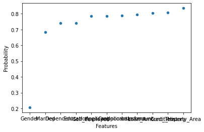
tbl_p = DataFrame(X_train.columns)
tbl_p['Probability'] = Series(p_x_val.flatten())
tbl_p.columns = ['Features','Probability' ]
tbl_p['Probability'] = sorted(tbl_p['Probability'])
tbl_p
Out[15]:
Features Probability
0 Gender 0.206190
1 Married 0.683352
2 Dependents 0.742239
3 Education 0.742439
4 Self_Employed 0.786568
5 ApplicantIncome 0.787226
6 CoapplicantIncome 0.789256
7 LoanAmount 0.796142
8 Loan_Amount_Term 0.803901
9 Credit_History 0.807324
10 Property_Area 0.835503
In [16]:
ax = tbl_p.plot.scatter(x = 'Features', y = 'Probability')
In [17]:
# The actual prediction of the target variable for X_train
y_train_pred = model.predict(X_train)
y_train_pred
Out[17]:
array([1, 1, 1, 1, 1, 1, 1, 0, 1, 1, 1, 1, 1, 1, 1, 1, 1, 0, 1, 1, 0, 1,
       0, 0, 1, 1, 1, 1, 1, 1, 1, 1, 1, 1, 1, 1, 0, 1, 1, 1, 1, 1, 1, 1,
       1, 1, 1, 1, 0, 1, 1, 1, 1, 1, 0, 1, 1, 1, 1, 1, 1, 1, 0, 0, 0, 1,
       0, 1, 1, 0, 1, 1, 1, 0, 1, 1, 1, 1, 0, 1, 1, 1, 1, 1, 1, 1, 1, 1,
       1, 1, 1, 1, 1, 1, 1, 1, 1, 1, 1, 1, 1, 1, 1, 1, 1, 1, 1, 1, 0, 1,
       1, 1, 0, 1, 1, 1, 1, 1, 1, 1, 1, 1, 0, 1, 1, 1, 1, 1, 0, 1, 0, 1,
       1, 1, 1, 1, 1, 1, 0, 1, 1, 1, 1, 1, 1, 1, 1, 1, 1, 1, 0, 1, 1, 1,
       1, 0, 1, 1, 1, 1, 1, 1, 0, 1, 1, 1, 1, 1, 0, 1, 1, 1, 1, 1, 1, 1,
       1, 0, 1, 0, 0, 1, 1, 1, 1, 1, 0, 1, 1, 1, 1, 1, 1, 1, 1, 1, 1, 1,
       1, 1, 1, 0, 1, 1, 1, 1, 1, 1, 1, 1, 1, 0, 1, 1, 1, 1, 1, 1, 0, 1,
       0, 1, 1, 1, 1, 1, 1, 1, 1, 1, 1, 1, 1, 1, 1, 1, 1, 1, 1, 1, 1, 1,
       1, 1, 1, 1, 1, 1, 1, 1, 0, 1, 1, 1, 0, 1, 0, 1, 1, 1, 1, 1, 1, 1,
       1, 1, 1, 0, 1, 1, 1, 1, 1, 1, 1, 1, 1, 1, 1, 1, 0, 1, 1, 1, 1, 1,
       1, 1, 1, 1, 1, 0, 1, 0, 1, 1, 1, 1, 1, 1, 0, 1, 1, 1, 1, 1, 1, 0,
       1, 1, 1, 1, 1, 1, 1, 1, 1, 1, 1, 1, 1, 1, 1, 1, 1, 0, 0, 1, 1, 1,
       1, 1, 1, 1, 1, 1, 1, 1, 0, 1, 1, 1, 1, 1, 1, 1, 0, 1, 1, 1, 1, 1,
       1, 0, 1, 1, 1, 1, 0, 1, 1, 1, 1, 1, 1, 1, 1, 0], dtype=int64)
In [18]:
# actual y_train values
np.array(y_train)
Out[18]:
array([1, 0, 1, 1, 1, 1, 1, 0, 1, 0, 1, 1, 1, 0, 1, 1, 1, 0, 0, 1, 0, 1,
       0, 0, 0, 1, 1, 1, 0, 1, 0, 0, 0, 1, 0, 1, 0, 1, 1, 1, 0, 1, 1, 1,
       1, 1, 1, 1, 0, 1, 1, 1, 0, 0, 0, 1, 1, 0, 1, 1, 1, 1, 0, 0, 0, 0,
       0, 1, 1, 0, 1, 1, 1, 0, 1, 0, 0, 0, 0, 1, 1, 1, 0, 0, 1, 1, 1, 1,
       1, 1, 1, 1, 1, 1, 1, 0, 1, 1, 1, 1, 1, 1, 1, 1, 1, 1, 1, 0, 0, 1,
       1, 1, 0, 1, 1, 1, 1, 1, 0, 1, 1, 1, 1, 1, 1, 1, 1, 1, 0, 0, 1, 1,
       1, 1, 1, 0, 0, 1, 0, 0, 0, 1, 1, 1, 1, 1, 1, 1, 0, 1, 0, 1, 0, 0,
       1, 1, 1, 1, 1, 1, 1, 0, 0, 1, 1, 1, 0, 1, 0, 1, 1, 1, 0, 1, 0, 1,
       1, 0, 1, 0, 0, 0, 1, 0, 1, 1, 0, 1, 1, 1, 1, 0, 0, 1, 1, 0, 1, 1,
       1, 0, 1, 1, 0, 1, 1, 1, 1, 1, 1, 0, 0, 0, 1, 1, 1, 1, 0, 1, 0, 1,
       0, 1, 1, 1, 1, 0, 0, 1, 1, 1, 1, 1, 1, 1, 1, 1, 0, 1, 1, 1, 1, 0,
       1, 1, 1, 0, 1, 1, 1, 1, 0, 0, 1, 1, 0, 1, 0, 0, 0, 0, 1, 1, 0, 1,
       1, 1, 1, 1, 0, 1, 1, 1, 1, 1, 1, 1, 1, 1, 1, 1, 0, 1, 1, 1, 0, 1,
       0, 1, 1, 1, 1, 0, 1, 0, 1, 1, 1, 1, 0, 0, 0, 1, 1, 1, 1, 0, 1, 0,
       0, 1, 1, 1, 1, 1, 0, 1, 1, 1, 1, 0, 1, 1, 1, 1, 1, 0, 1, 1, 0, 1,
       1, 1, 1, 1, 1, 1, 1, 1, 0, 1, 0, 0, 1, 1, 1, 1, 0, 1, 1, 1, 1, 0,
       1, 0, 1, 1, 1, 0, 0, 1, 0, 1, 1, 1, 1, 0, 0, 0], dtype=int64)
In [19]:
print('Actual y_train values: \n', Counter(y_train))
print('Predicted y_train values: \n', Counter(y_train_pred))
Actual y_train values: 
 Counter({1: 253, 0: 115})
Predicted y_train values: 
 Counter({1: 319, 0: 49})
In [20]:
confusion_matrix(y_train, y_train_pred)
Out[20]:
array([[ 43,  72],
       [  6, 247]], dtype=int64)
In [21]:
# Precision = TP/(TP+FP) for training dataset
Precision = 247/(247+72)
Precision
Out[21]:
0.774294670846395
In [22]:
# Recall = TP/(TP+FN) for training dataset
Recall = 247/(247+6)
Recall
Out[22]:
0.9762845849802372

Searching the Key Hyperparameters

In [23]:
solvers = ['newton-cg','lbfgs','liblinear']
penalty = ['l2']
c_val = [100, 10, 1.0, 0.1, 0.01]
grid = dict(solver = solvers, penalty = penalty, C = c_val)
cv = RepeatedStratifiedKFold(n_splits = 10, n_repeats = 3, random_state = 1)
grid_search = GridSearchCV(estimator = model, param_grid = grid, n_jobs = -1, cv = cv,scoring = 'accuracy', error_score = 0)
grid_result = grid_search.fit(X_validation, y_validation)
print("Best: %f using %s" %(grid_result.best_score_, grid_result.best_params_))
means = grid_result.cv_results_['mean_test_score']
stds = grid_result.cv_results_['std_test_score']
params = grid_result.cv_results_['params']
for mean, stdev, param in zip(means, stds, params):
    print("%f (%f) with %r" % (mean, stdev, param))
Best: 0.845726 using {'C': 100, 'penalty': 'l2', 'solver': 'newton-cg'}
0.845726 (0.108823) with {'C': 100, 'penalty': 'l2', 'solver': 'newton-cg'}
0.845726 (0.093113) with {'C': 100, 'penalty': 'l2', 'solver': 'lbfgs'}
0.842521 (0.098151) with {'C': 100, 'penalty': 'l2', 'solver': 'liblinear'}
0.839957 (0.103594) with {'C': 10, 'penalty': 'l2', 'solver': 'newton-cg'}
0.837179 (0.090634) with {'C': 10, 'penalty': 'l2', 'solver': 'lbfgs'}
0.837179 (0.090634) with {'C': 10, 'penalty': 'l2', 'solver': 'liblinear'}
0.831410 (0.077969) with {'C': 1.0, 'penalty': 'l2', 'solver': 'newton-cg'}
0.839530 (0.080277) with {'C': 1.0, 'penalty': 'l2', 'solver': 'lbfgs'}
0.834402 (0.086797) with {'C': 1.0, 'penalty': 'l2', 'solver': 'liblinear'}
0.714957 (0.069707) with {'C': 0.1, 'penalty': 'l2', 'solver': 'newton-cg'}
0.725855 (0.065177) with {'C': 0.1, 'penalty': 'l2', 'solver': 'lbfgs'}
0.730983 (0.072097) with {'C': 0.1, 'penalty': 'l2', 'solver': 'liblinear'}
0.679915 (0.043285) with {'C': 0.01, 'penalty': 'l2', 'solver': 'newton-cg'}
0.679915 (0.043285) with {'C': 0.01, 'penalty': 'l2', 'solver': 'lbfgs'}
0.679915 (0.043285) with {'C': 0.01, 'penalty': 'l2', 'solver': 'liblinear'}

Fine-tuning the Model

In [24]:
new_model = LogisticRegression(penalty ='l2',C = 100, solver = 'newton-cg').fit(X_train,y_train)
print("Old model score on Training set: \n", model.score(X_train, y_train))
print("New model score after tuning hyperparameter: \n", new_model.score(X_train, y_train))
Old model score on Training set: 
 0.7880434782608695
New model score after tuning hyperparameter: 
 0.7907608695652174
In [25]:
y_test_old = model.predict(X_test)
y_test_new = new_model.predict(X_test)

Model Diagnotics

In [26]:
print('Actual y_test values: \n', Counter(y_test))
print('Predicted y_test values with old model: \n', Counter(y_test_old))
print('Predicted y_test values with new model: \n', Counter(y_test_new))
Actual y_test values: 
 Counter({1: 84, 0: 39})
Predicted y_test values with old model: 
 Counter({1: 101, 0: 22})
Predicted y_test values with new model: 
 Counter({1: 104, 0: 19})
In [27]:
print("Precision score for old model: \n",precision_score(y_test, y_test_old))
print("Recall score for old model:\n", recall_score(y_test, y_test_old))
Precision score for old model: 
 0.7920792079207921
Recall score for old model:
 0.9523809523809523
In [28]:
print("Precision score for fine-tuned model: \n",precision_score(y_test, y_test_new))
print("Recall score for fine-tuned model:\n", recall_score(y_test, y_test_new))
Precision score for fine-tuned model: 
 0.7980769230769231
Recall score for fine-tuned model:
 0.9880952380952381

Conclusion

The default Logistic Regression model works well in training dataset, but in order to avoid overfitting, which will cause relatively more inaccuracy in prediction, it is bests to split up the training dataset and fine-tune the model on a validation dataset. After fine-tuning the hyperparameter, not only the model score improved, but also the precision score and recall score.